4 Types of SQL Joins for Database Tables

This post was written by Nicole Hitner, a content strategist at Exago, Inc., producers of embedded business intelligence for software companies. She manages the company’s content marketing, writes for their blog, and assists the product design team in continuing to enhance Exago BI.

SQL Joins Explained

A relational database is ultimately just a collection of data tables, each of which is useful on its own, but exponentially more useful when joined to its neighbors. Data scientists-to-be will have a leg up on the competition if they go into their first SQL course with a basic understanding of the four essential join types, which not only merge data on output but also filter it to display a specific subset of records. Before we explore how joins define the relationships between tables, however, we first need to understand what a key field is.

Key Fields

We will discuss two types of key fields: primary keys and foreign keys. A primary key is a field or column that uniquely identifies each row or record in the table. A table must have exactly one primary key to qualify as relational, but that key can be composed of multiple columns.

A foreign key, by contrast, is one or more fields or columns that corresponds to the primary key of another table. Foreign keys are what make it possible to join tables to each other.

In the set of tables below, for example, kid_id is the primary key for KIDS and chore_id is a foreign key corresponding to a field of the same name in CHORES. Note that CHORES does not have a foreign key for KIDS.

You might wonder why kid_name isn’t the primary key for the KIDS table. Its values are indeed unique per record, but what happens if we begin adding records to the table? As soon as a new, different Steve is added to the KIDS table, kid_name stops being unique per record. This is why it’s a good idea for the primary key to have only one job: locating records.

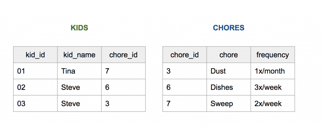
Because KIDS has a foreign key corresponding to a primary key in CHORES (chore_id), we know that we can join these two tables together to make one. How that happens, however, will depend on the join type.

Full Outer Joins

The most basic database join is what’s known as a full outer join. The output contains all the primary ids in both tables and all fields in both tables, regardless of whether the records have matches in the opposite table. If, in the diagram below, we represent data that will appear in the output using the color blue, we can see that all records from both tables will be returned.

Let’s look at a new example. Consider the following tables found in a university database.

If we do a full outer SQL join on rm_id, keeping all primary ids in both tables as well as all columns, ordering by course_id ascending, we end up with the following output:

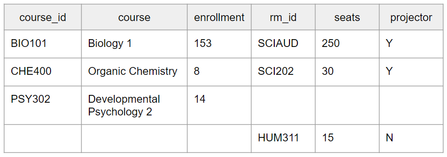
Because Developmental Psychology 2 has not yet been assigned a room, it does not have a match in the ROOM table. HUM311 has likewise not been assigned a course, so it has no match in the COURSE table. As a result, there are lots of null or empty values in the output, and this is fairly typical of full outer joins. The goal is to be all-inclusive, which isn’t the case for other join types. If, for example, we were only interested in courses with rooms, we might use a left outer join instead.

Get To Know Other Data Science Students

Sunil Ayyappan

Senior Technical Program Manager (AI) at LinkedIn

Read Story

Ginny Zhu

Data Science Intern at Novartis

Read Story

Meghan Thomason

Data Scientist at Spin

Read Story

Left and Right Outer Joins

Left outer joins use all the primary ids of the left table and all fields of both tables. In the diagram below, we see that all records of the left table appear in the output, along with those in the right table, as long as they have matches in the left.

Referring back to our collegiate example, a left outer join of the two original tables would yield the following:

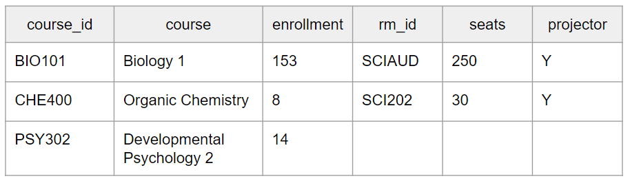
Note that HUM311 is nowhere to be found on this table. That is because it neither has a primary key in the left table (because it’s a room, not a course) nor is it associated with a course. We’re beginning to see how joins can act as filters by restricting which records return from the query.

The mirror opposite of a left outer join is, as you might have guessed, a right outer join. In a right outer join, all the primary ids of the right table appear in the output along with all columns from both tables.

This time, it’s the PSY302 class that doesn’t make the cut.

All the rooms automatically make it into the output, but the only courses that will be returned, in this case, are those with rooms assigned. PSY302 has not yet been assigned a room and is therefore excluded from the resulting table.

Inner SQL Joins

The fourth and final basic join type is an inner join. Here, the only records we want to be returned on output are those referenced in both tables.

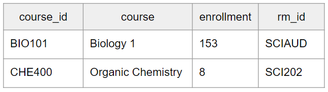
So, in our courses and rooms example, courses without rooms are out, as are rooms without courses. This leaves us with just the science courses and their respective rooms:

Semi Joins and Anti Joins

Inner, left outer, right outer, and full outer are the four basic join types you should know when you’re just getting into SQL, but there are other, less common joins to explore as well. Semi joins, unlike the joins we’ve looked at so far, don’t return all columns of both tables. Instead, they just return the columns of the left table and records with matches in the right table. If we were to diagram this concept, it might look something like this:

The output would look similar to the output resulting from an inner join, except columns specific to Table B (ROOM) would be missing:

An anti join is the opposite of a semi join; we only return records from Table A that do not have matches in Table B.

Since only the Psychology course has no assigned room, it would be the only record to appear on output:

Once you’ve got these basic join types down pat, you can explore formulaic joins, such as those containing conditional statements, ranges, and calculations! SQL is such a versatile language that joining options are virtually endless. Understanding these four primary concepts will help prepare you for other lessons in databases, data science, and analytics. Moreover, SQL is extremely important in the field of data science. As a result, data scientists should have a solid foundation in SQL to handle structured data.