Linear Regression Algorithm is a machine learning algorithm based on supervised learning. We have covered supervised learning in our previous articles.
Here we are going to focus on Linear regression. Linear regression is a part of regression analysis. Regression analysis is a technique of predictive modeling that helps you to find out the relationship between Input and the target variable.
Regression analysis is used for three types of applications:
- Finding out the effect of Input variables on Target variable.
- Finding out the change in Target variable with respect to one or more input variable.
- To find out upcoming trends.
Here are the types of regressions:
- Linear Regression
- Multiple Linear Regression
- Logistic Regression
- Polynomial Regression
What is Linear Regression?
Linear regression is one of the very basic forms of machine learning in the field of data science where we train a model to predict the behaviour of your data based on some variables. In the case of linear regression as you can see the name suggests linear that means the two variables which are on the x-axis and y-axis should be linearly correlated.
An example is let’s say you are running a sales promotion and expecting a certain number of count of customers to be increased now what you can do is you can look the previous promotions and plot if over on the chart when you run it and then try to see whether there is an increment into the number of customers whenever you rate the promotions and with the help of the previous historical data you try to figure it out or you try to estimate what will be the count or what will be the estimated count for my current promotion this will give you an idea to do the planning in a much better way about how many numbers of stalls maybe you need or how many increase number of employees you need to serve the customer. Here the idea is to estimate the future value based on the historical data by learning the behaviour or patterns from the historical data.
Get To Know Other Data Science Students

Jonas Cuadrado
Senior Data Scientist at Feedzai

Melanie Hanna
Data Scientist at Farmer's Fridge

Sunil Ayyappan
Senior Technical Program Manager (AI) at LinkedIn
In some cases, the value will be linearly upward that means whenever X is increasing Y is also increasing or vice versa that means they have a correlation or there will be a linear downward relationship.
One example for that could be that the police department is running a campaign to reduce the number of robberies, in this case, the graph will be linearly downward.
Linear regression is used to predict a quantitative response Y from the predictor variable X.
Mathematically, we can write a linear regression equation as:

Where a and b given by the formulas:

Here, x and y are two variables on the regression line.
b = Slope of the line.
a = y-intercept of the line.
x = Independent variable from dataset
y = Dependent variable from dataset
Use Cases of Linear Regression:
- Prediction of trends and Sales targets – To predict how industry is performing or how many sales targets industry may achieve in the future.
- Price Prediction – Using regression to predict the change in price of stock or product.
- Risk Management- Using regression to the analysis of Risk Management in the financial and insurance sector.
Let’s move to implementation of linear regression algorithm in our sample dataset.
The dataset that we are using has below columns –
| Hyundai(Thousands of dollars) | Maruti (Thousands of dollars) | Mahindra (Thousands of dollars) | Sales(Thousands of dollars) | |
| 1 | 230.1 | 37.8 | 69.2 | 22.1 |
| 2 | 44.5 | 39.3 | 45.1 | 10.4 |
| 3 | 17.2 | 45.9 | 69.3 | 9.3 |
| 4 | 151.5 | 41.3 | 58.5 | 18.5 |
| 5 | 180.8 | 10.8 | 58.4 | 12.9 |
In our data Frame, the first column is an index column and the first row is the column header. Our dataset has 200 rows. Let’s describe the dataset:
- Hyundai – This column indicates the money spent on advertising the Hyundai cars in the given market.
- Maruti – Similarly, money spent on advertising by Maruti car.
- Mahindra – Similarly, money spent on advertising by Mahindra car.
- Sales – This column indicates the sales of cars in the given market. (Value of the sales in thousands)
Implementation of linear regression:
For our implementation, we are using Jupyter Notebook and executing our algorithm in python v3.0.
- Let us start by loading the necessary libraries. Firstly, we are importing Pandas which is the most popular python library for data exploration, manipulation and analysis. Please follow this document to install Pandas. We are importing Mathplotlib for multiplatform data visualization. For linear regression, we need to use Statsmodels to estimate the model coefficients for the advertising data.

2. Next steps we are going to load the dataset, read the data into a data frame and display the head (top 5 rows). Also, we can see the total number of rows. There are 200 observations in the given dataset.

3. Let’s visualize the relationship between the features and the sales response using scatterplots.
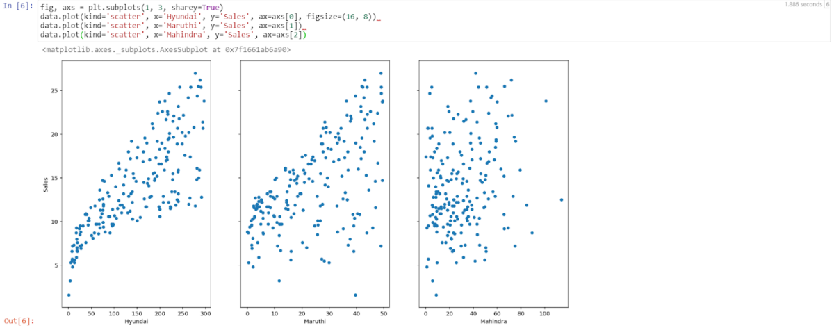
Now by looking into the above scatterplots we can easily say that Hyundai advertising and sales have a strong relationship. However, Maruti’s and Mahindra’s datapoints look scattered all over the graph that implies that they have a weak relationship between advertisement and sales.
4. Now let’s Estimate the model coefficients for Linear Regression by using single feature to predict quantitative response. It takes the following form:

Where y will be the response
X will be the feature
a is the intercept
b is the coefficient for x, a & b are called Model coefficient.
To calculate coefficients, we will use the least square criterion, which means we will find a line that will decrease the sum of squared errors.
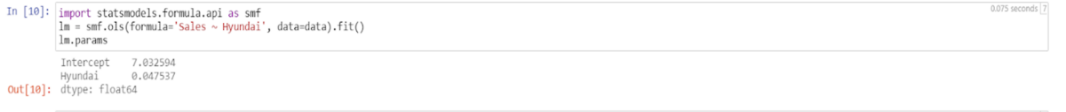
In this step we will load statsmodels to estimate the model coefficients for the advertising data. Statsmodels allows users to fit statistical models by importing OLS. As shown below we are going to fit the model using statsmodels OLS.
Here we are finding the model coefficient between Sales column and Hyundai column. lm.params will print the coefficient.
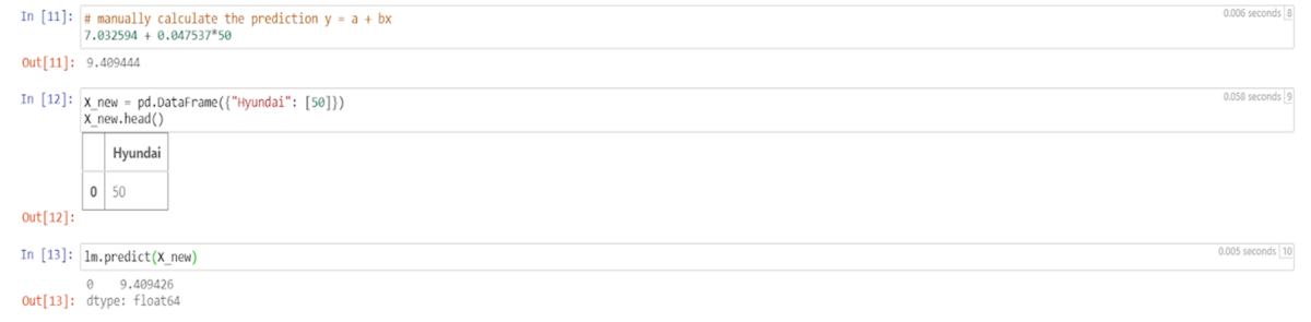
5. From step 4- we got the value of A and B. we will use the model to predict the future sales of Hyundai cars. Let’s say in the new market Hyundai is spending 50 thousand dollars in advertising. That means the new value of X will be 50. Now using Y = A + BX to predict the new value.
6. Now let’s plot the least square line by creating a data frame with the minimum and maximum
values of Hyundai and predict for x value and store that value in preds variable.

7. Let’s plot the observed data graph and the least square line using preds value and new x value.
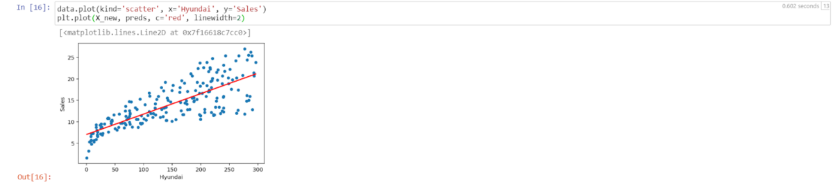
In linear regression, the observation blue dots are assumed to be the result of random deviation from an underlying relationship (red line) between a dependent variable (y) and an independent variable (x). Here the goal is to decrease the distance between the red line and the blue dots. If all the blue dots are on red lines that means Root means square error will low and better.
However, Linear Regression is a very vast algorithm and it will be difficult to cover all of it. At the same time, every data scientist should be well-versed in this algorithm. You can improve the model in various ways could be by detecting collinearity and by transforming predictors to fit nonlinear relationships. This article is to get you started with simple linear regression. Let’s quickly see the advantage and disadvantage of linear regression algorithm:
- Linear regression provides a powerful statistical method to find the relationship between variables. It hardly needs further tuning. However, it’s only limited to linear relationships.
- Linear regression produces the best predictive accuracy for linear relationship whereas its little sensitive to outliers and only looks at the mean of the dependent variable.
Since you’re here…Are you interested in this career track? Investigate with our free guide to what a data professional actually does. When you’re ready to build a CV that will make hiring managers melt, join our Data Science Bootcamp which will help you land a job or your tuition back!