Introduction to Regression and Classification in Machine Learning

In my last post, we explored a general overview of data analysis methods, ranging from basic statistics to machine learning (ML) and advanced simulations. It was a pretty high-level overview, and aside from the statistics, we didn’t dive into much detail. In this post, we’ll take a deeper look at machine-learning-driven regression and classification, two very powerful, but rather broad, tools in the data analyst’s toolbox.

As my university math professors always said, the devil is in the details. While we will look at these two subjects in more depth, I don’t have programming examples for you. We’ll go over how the methods work and a couple of examples. We’ll look at some pros and cons, and we will talk about a couple of important issues when using machine learning. But you’ll need to learn a little programming and debug your code to interpret your results.

Modern data analysis is fundamentally computer-based. Could you do these calculations by hand? Probably. But it would take a very long time, and it would be extremely tedious. That means you’ll probably need some programming skills to accomplish classification or regression tasks.

However, don’t let coding scare you away from the tutorial. If you have any contact with machine learning, these basics are important to understand, even if you never write a line of code.

Now, let’s get started.

Background

Types of Machine Learning

There are two main types of machine learning: supervised and unsupervised. Supervised ML requires pre-labeled data, which is often a time-consuming process. If your data isn’t already labeled, set aside some time to label it. It will be needed when you test your model.

By labeling, I mean that your data set should have inputs and the outputs should already be known. For example, a supervised regression model that determines the price of a used car should have many examples of used cars previously sold. It must know the inputs and the consequent output to build a model. For a supervised classifier that, for example, determines whether a person has a disease, the algorithm must have inputs and it must know which output those inputs led to.

Unsupervised ML requires no initial labeling from the data scientist. There is a kind of label “out there in the ether,” we just can’t see it. Unsupervised algorithms are complex to implement and generally require a lot of money and data. The algorithm receives no guidance from the data scientist, like: Patient 1 with symptoms A, D, and Z has cancer, while Patient 2 with symptoms A, D, and –Z does not.

When the general public thinks of artificial intelligence, they think of (very good) unsupervised ML algorithms. Their power lies in their ability to learn on their own and to make connections in higher-dimensional vector spaces. That phrase may sound intimidating, but it really just means the algorithms can look at multiple connections at once and discover insights that we humans, with our limited memories, would miss. They might make connections humans cannot understand, too, leading to black box algorithmic decisions. More on that later.

Regression and Classification

In the last article, I discussed these a bit. Classification tries to discover into which category the item fits, based on the inputs. Regression attempts to predict a certain number based on the inputs. There’s not much more to it than that at the surface level.

Splitting Data Sets

When we train a ML model, we need to also test it. Because data can be expensive and time-consuming to gather, we often split the (labeled) data set we have into two sections. One is the training set, which the supervised algorithm uses to adjust its internal parameters and make the most accurate prediction based on the inputs.

The remainder of the data set (usually around 30%) is used to test the trained model. If the model is accurate, the test data set should have a similar accuracy score to that of the training data. However, we often see underfitting or overfitting of the model, and that will become apparent in the testing stage.

For now, it’s sufficient to know that this “training-test split” is a very common evaluation method in ML-based data science.

Common Tools

There are many tools for data analysts, some more popular than others. This is a nice introduction. And while it doesn’t cover all tools (the list would be enormous), it does touch on many of the popular ones.

Languages like R and Python are very common, and if you look at any data science course, you’re likely to see some mention of Python libraries like scikit-learn, pandas, and numpy. There is, fortunately, a large online community to help you learn these tools, and I strongly recommend starting out with a high-level language like Python, especially if you have little programming background.

Regression

Now that we have the preliminaries out of the way, let’s start looking at some regression techniques.

Least Squares

The concept is straightforward: we try to draw a line through the data set and measure the distance from each point to the line. The distance is termed the error, and we add up all these errors. Then we draw another, slightly different line, add up all the errors, and, if the second line has a lower total error than the first one, we use the second line. This process is repeated until a line with the lowest error is found.

The name of the method derives from its formula, which actually squares the error value. This is because points above the line would offset points below the line (positive plus negative goes to zero). Squared values always give a positive number, so we can be sure that we are always adding positive numbers together.

Least squares regression will produce some linear equation, like:

car price = 60,000 – 0.5 * miles – 2200 * age (in years)

Every two miles driven reduces your sale price by $1, and every year of ownership reduces it a further $2,200. So a 5-year-old car with 50,000 miles will sell for $24,000. This assumes a brand new vehicle, with zero miles and zero years, costs $60,000. Whether this reflects reality is suspect, but this example illustrates the basic equation produced by the least squares method.

Least squares is very helpful when you have a linear relationship. It doesn’t have to be in two dimensions, as our example above illustrates. Technically our car example would use a predictor plane instead of a predictor line, and higher dimensions (i.e., more variables) would result in hyperplane predictors. Species of a three-dimensional world, we cannot easily visualize hyperplanes geometrically. However, the idea remains: if a simple linear relationship can be found, linear regression is applicable.

Least squares is also a common first approach because it’s very cheap in terms of computing power. However, this efficiency comes with the cost of not being useful on relationships that are not linear in nature—which is actually many relationships.

Non-linear regressors like polynomial and logarithmic ones still use the least squares method, but shift from producing a line (or linear plane or hyperplane) to a polynomial curve or polynomial surface. A cubic function for car prices might look like:

car price = 60,000 – 0.01 * miles³ + 0.3 * miles² * years – 3.5 * miles * years² + … – 0.94 * years³

I completely made up that equation, but you can see that to reach higher dimensional polynomials we just multiply variables together. The machine finds the constant factors (0.01, 0., 3.5, 0.94 in our example).

k-Nearest Neighbors (KNN) Regression

The k-nearest neighbors approach is intuitively more closely associated with classification, but it can be used for regression as well. If you remember the discussion about continuous and categorical variables in my last post, the line isn’t always clear (recall the checking account example). If we break down a continuous output into multiple categories, we can apply classifier models to generate regression-like predictors.

Pure KNN regression simply uses the average of the nearest points, using whatever number of points the programmer decides to apply. A regressor that uses five neighbors will use the five closest points (based on input) and output their average for the prediction.

I will discuss k-nearest neighbors more later, because it fits better with classification, but know that it can be used for regression purposes.

Sanity Checking Your Model

Sometimes we get so caught up in the programming and error rates and accuracy scores, we go a bit insane. ML requires quite a bit of tinkering, and when we start to see improvements, we get very excited. If you started out with 70% baseline accuracy and tweaked and tweaked and finally got to 80%, you must be doing something right, right? Well, maybe not.

Your data set might really have a 50-50 chance of outcome A or outcome B, and your original regressor was guessing too systematically. To ensure we can trust the results, it’s a good idea to use a dummy regressor. These will predict outcomes based on predetermined rules that are not connected to your data at all. If your dummy regression is producing similar results to your trained regressor, you haven’t made any true progress or insights. Common dummy regressors predict a value by the mean, the median, or a quantile. Your data set might not actually need machine learning insights if these dummy regressors are sufficient, or you might need a new approach.

Classification

Classification attempts to classify a data point into a specific category based on its features or characteristics. Based on measurements, what is this plant? What kind of worker will someone be based on the answers to a personality test? Using solely color variation, which bananas are ripe, which are underripe, and which are overripe?

As you may have concluded, classification questions are usually “what kind of…” while regression questions are usually “how much …” or “what is the probability that …”. These are not always mutually exclusive. But this is a good rule of thumb to help you determine whether your problem will require a classification or regression model.

Linear Support Vector Machines (SVMs)

In its simplest form, SVMs closely resemble least squares regression. In least squares, we tried to find the line that minimized the error term. With an SVM, we look for a line that fits between the two classes, then we try to expand that line as wide as possible. The line that can expand the farthest is considered our decision line. Points on one side are Class A and points on the other side are Class B.

This visual might help:

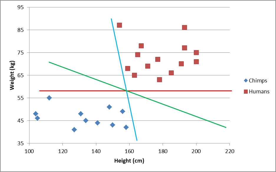
All these lines can separate the two classes (chimps and humans), but some lines are probably better classifier lines than others. The blue one is heavily dependent on height, so slightly taller chimps or slightly shorter humans may be classified incorrectly. The red line is horizontal and therefore entirely dependent on weight. Extra-heavy chimps (say 62 kg.) will be incorrectly classified as human. The green one seems to take both factors into account.

SVM will take each guess and try to widen it. The line that can be widened the most before it touches a data point is considered the best classifier. Intuitively, it is the decision line that has the greatest buffer between data points and the decision criteria.

Out of our choices, the green one can expand the most without touching a data point:

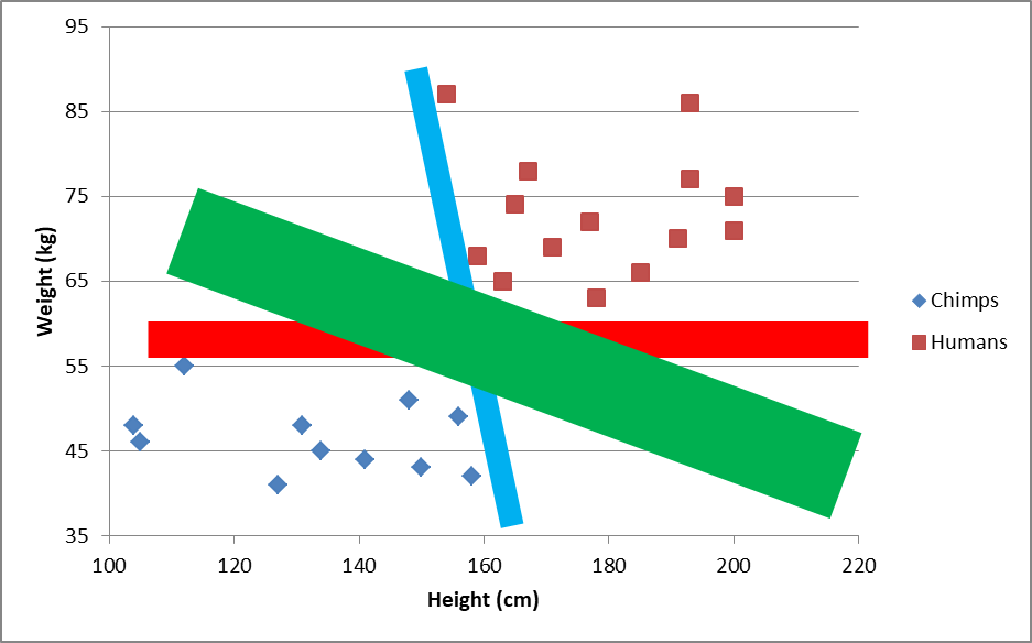
If a SVM algorithm could only choose from these three lines, it would choose green. Note that the decision line will be the thin line from the first graph. Technically, the green “line” in the second graph is a rectangle. A real SVM will test hundreds or thousands of lines.

Non-Linear SVMs

Linear classifiers are great because they’re cheap in terms of compute power and compute time. That means they can easily scale to mammoth data sets. However, sometimes linear classifiers just don’t conform to the data. In these cases, you might want to try a different kernel, often a radial kernel. This means instead of drawing lines, you draw circle-like decision boundaries.

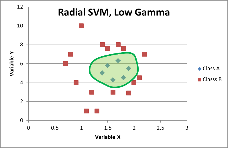
Here, the green spline represents the radial basis SVM and all points inside the shaded area will be predicted as Class A. It isn’t a circle centered at the center of the group. It is actually multiple circles drawn together, each radiating out from the data points. My drawing isn’t perfect, but the concept should be understandable: draw circles out from data points and then put them together to get the decision line that offers the widest buffer between Class A and Class B data points.

SVMs with polynomial kernels are also popular, wherein polynomial lines are used instead of circles or straight lines. And while we only looked at problems with two inputs (height and weight, X and Y), SVMs can easily take more inputs.

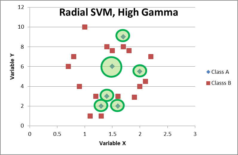
When writing the code, there are multiple parameters you can set. Especially important is gamma, which is particularly noticeable with radial-basis SVMs. The higher your gamma parameter, the tighter the circles are around the data points. High gammas might lead to tight circular boundaries that isolate individual data points, but this is extremely overfit and will not classify new data well.

Decision Tree Classifiers (DTCs)

Let’s look at a different kind of classifier. Decision trees recursively split up the data points into groups (nodes). Each node is a subset of the node above, and if the decision tree is a good classifier, the accuracy of predictions improves as it moves down the branches. Decision trees can achieve extremely high accuracies on the first attempt. However, be cautious about such high accuracy rates, because decision trees are notorious for overfitting the training data. You might get 95% accuracy on your training set then get 65% on your test set.

To illustrate, a decision tree might look like this:

We start with 100 samples, and the tree breaks down the groups multiple times. At the beginning, we have labels for 20 bicycles, 10 unicycles, 30 trucks, 10 motorcycles, and 30 cars. The classifier splits the data points up by their attributes. A classifier doesn’t ask questions like “how many wheels does it have”, but it will mathematically consider that Data Point 1 has two wheels and one motor while Data Point 2 has one wheel and zero motors.

If all the data points in a node are the same class, the DTC doesn’t have to split it anymore, and that branch of the tree will terminate. These are called pure nodes. Conversely, if the node contains samples of more than one class, it could be split further. However, we do not want to split nodes continually if it makes the model excessively complex.

There are two parameters commonly adjusted when trying to train the best DTC: maximum number of nodes and depth.

Depth refers to how many times the DTC should split up the data. If you set the maximum depth to three, the DTC will only split subsets three times, even if the ending nodes are not pure. Of course, the DTC tries to split the data such that the purity of the end nodes are as high as possible.

The maximum number of nodes is the upper limit on how many nodes there are in total. If you set this to four, there can only be four subsets. That could manifest in a depth of one, where the original set is split into four subsets right away. It could also be a depth of two, where the original splits into two subsets, and one of the subsets is itself split into two further subsets.

To reduce overfitting, the maximum depth parameter is usually adjusted. This stops the DTC from continuing to split the data sets even when accuracy is high enough.

Random Forests

The law of large numbers is a central theme in probability and statistics. This idea flows over into data science, and having more samples is often viewed as better. Because DTCs can overfit very easily, sometimes we use a set of trees, which would be a forest. Hence the name random forest classifiers (RFCs), is a collection of DTCs with randomly selected data from the training set.

In the code, the data scientist would choose a maximum depth, maximum nodes, minimum samples per node, and other parameters for each tree, plus how many trees and features (input variables) to use. Then the algorithm builds trees using different subsets of the training data set. This is done to avoid biases.

To make the RFC more random, you can also choose a subset of features. For instance, if there are 10 features and maximum_features = 7, the trees will only choose seven of the features. This prevents strongly influential features from dominating every tree and makes the forest more diverse.

The final model is a combination of those trees. If there are 30 trees in the forest and 20 trees predict Class A and 10 predict Class B, the RFC will call that data point Class A.

Cleary, RFCs are more robust because they take a sample of multiple trees. The two drawbacks are computing power required and the black box problem.

Since your model has to generate multiple DTCs, it has to process and reprocess the training data repeatedly. Then, once a model is settled, every new data point must be run through all the DTCs to make a decision. Depending on the dimensions of your data, the size of your data set, and the complexity of your RFC, this could require quite a bit of computing power. However, because each tree in the forest is independent, a RFC can easily be parallelized. If you’re working with GPUs, the computation burden might not actually be that bad.

The other issue, black box algorithms, is a major focus of computer science, philosophy, and ethics. In a nutshell, the black box problem is our (humans’) inability to decipher why a decision is reached. This happens frequently in RFCs because there are so many DTCs. Though this can also happen with larger trees, it’s usually easier to visualize how a DTC reaches its conclusion. A 200-tree, depth-20 forest is much harder to decipher.

Neural Networks

The last classifier I will discuss is neural networks. This is probably the hottest data science topic in popular culture. Neural networks are modeled after the human brain and are extremely powerful without much need for tuning the model. Their implementations are very complex, and they too suffer from the black box problem.

In neuroscience, thought and action are determined by the firing of neurons. Neurons fire based on their inner electrochemical state. Once a specific threshold is reached, the neuron “fires,” causing other neurons to react. This is the basis of neural networks.

Neural networks are layered sets of nodes, where input nodes send signals to nodes in a hidden layer, which in turn send signals to a final output. Every input node is connected to every hidden node, and every connection has its own weight. For example, Feature X might influence Hidden Node 1 by 0.5, while Feature X influences Hidden Node 2 by 0.1.

If the hidden node reaches its threshold, it propagates forward a signal. This could be to another hidden layer, or it could be to the output.

This illustration should be helpful in understanding the concept (yes, I painstakingly made it in Excel):

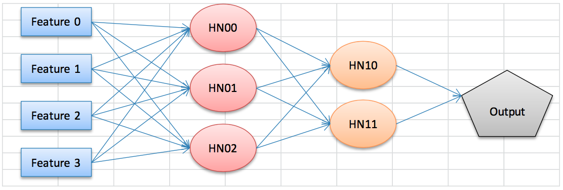
This neural network has four features and two hidden layers, the first with three nodes and the second with two nodes. Each one of the arrowed lines carries a weight, which will impact the node it points to. Sophisticated neural networks might have hundreds of nodes and several hidden layers.

To understand how these work better, let’s look at an example. This is clearly contrived, and activation functions—the formula determining whether a node fires—are usually much more complex. But this should get the point across:

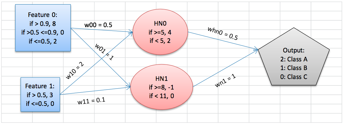
Now, if we have an input set of {2, 1}, 2 will enter the Feature 0 node and send 4 to HN0 and 8 to HN1. The Feature 1 node will send 6 to HN0 and 0.3 to HN1. The hidden layer, in turn, sends 4*0.5=2 and -1*1 = -1 to the output. 2 + (-1) = 1, so an input set of {2,1} should correspond to Class B.

These weights and signals are adjusted until the resultant data set matches the expected predictions as closely as possible. Bleeding edge approaches might put two neural networks in competition, send signals backward through the network, and do other clever operations to improve prediction ability.

The three disadvantages of neural networks are a voracious appetite for data, memory usage, and the black box problem.

Neural networks tend to perform best when they have huge amounts of input data, often on the levels that only Big Tech commands. Google and Facebook (among others) have far more data than any smaller organization could possibly own, and therefore they have the best algorithms. If your project is sparse on data, a neural network might not be a good idea.

Then, because the layers are not independent, a lot of information must be stored in working memory. Hard drives are cheap, but RAM is not. Yet neural networks can consume significant amounts of RAM.

And, as you can probably guess from just my illustrations, these get complicated fast. When there are five hidden layers, each with 100 nodes, and there is back propagation occurring, humans may have a difficult time understanding the why of the decision. Some tools and clever programming can help, though.

Ending Remarks

I hope you have learned a little about machine learning for regression and classification. There is plenty more to learn, and this is just a first-step introduction. There are many online courses to teach you the programming and practical details, as well as some good classes on the mathematics that support all of these algorithms.

Remember that machine learning is just computers doing math, not magical spells that pull insights out of nowhere. ML is an awesome tool—and I mean that in both senses: cool, but also so powerful that it inspires awe. Use it wisely and reap great benefit.

Since you’re here…
Curious about a career in data science? Experiment with our free data science learning path, or join our Data Science Bootcamp, where you’ll get your tuition back if you don’t land a job after graduating. We’re confident because our courses work – check out our student success stories to get inspired.